pacman::p_load(sf, spdep, tmap, tidyverse)Hands-on Exercise 2 : Global Measures of Spatial Autocorrelation
Overview
In this hands-on exercise, we explore how to compute Global and Local Measure of Spatial Autocorrelation (GLSA) by using spdep package.
Getting Started
The code chunk below install and load spdep, sf, tmap and tidyverse packages into R environment.
Getting the Data Into R Environment
Import shapefile into r environment
The code chunk below uses st_read() of sf package to import Hunan shapefile into R.
hunan <- st_read(dsn = "data/geospatial",
                 layer = "Hunan")
Reading layer `Hunan' from data source
`D:\zhphyo\ISSS624\Hands-on_Ex2\data\geospatial' using driver `ESRI Shapefile'
Simple feature collection with 88 features and 7 fields
Geometry type: POLYGON
Dimension: XY
Bounding box: xmin: 108.7831 ymin: 24.6342 xmax: 114.2544 ymax: 30.12812
Geodetic CRS: WGS 84Import csv file into r environment
Import Hunan_2012.csv into R by using read_csv() of readr package
hunan2012 <- read_csv("data/aspatial/Hunan_2012.csv")Rows: 88 Columns: 29
── Column specification ────────────────────────────────────────────────────────
Delimiter: ","
chr (2): County, City
dbl (27): avg_wage, deposite, FAI, Gov_Rev, Gov_Exp, GDP, GDPPC, GIO, Loan, ...
ℹ Use `spec()` to retrieve the full column specification for this data.
ℹ Specify the column types or set `show_col_types = FALSE` to quiet this message.Performing relational join
The code chunk below will be used to update the attribute table of hunan’s SpatialPolygonsDataFrame with the attribute fields of hunan2012 dataframe.
hunan <- left_join(hunan,hunan2012) %>%
  select(1:4, 7, 15)
Joining with `by = join_by(County)`Visualising Regional Development Indicator
prepare a basemap and a choropleth map showing the distribution of GDPPC 2012 by using qtm() of tmap package.
equal <- tm_shape(hunan) +
  tm_fill("GDPPC",
          n = 5,
          style = "equal") +
  tm_borders(alpha = 0.5) +
  tm_layout(main.title = "Equal interval classification")

quantile <- tm_shape(hunan) +
  tm_fill("GDPPC",
          n = 5,
          style = "quantile") +
  tm_borders(alpha = 0.5) +
  tm_layout(main.title = "Equal quantile classification")

tmap_arrange(equal,
             quantile,
             asp=1,
             ncol=2)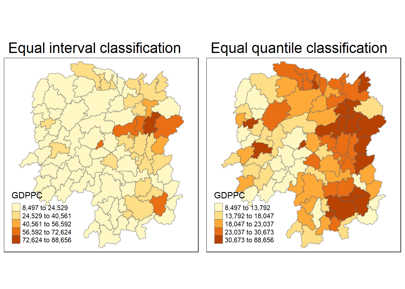
Global Spatial Autocorrelation
Computing Contiguity Spatial Weights
In the code chunk below, poly2nb() of spdep package is used to compute contiguity weight matrices for the study area. This function builds a neighbours list based on regions with contiguous boundaries. If you look at the documentation you will see that you can pass a “queen” argument that takes TRUE or FALSE as options. If you do not specify this argument the default is set to TRUE, that is, if you don’t specify queen = FALSE this function will return a list of first order neighbours using the Queen criteria.
More specifically, the code chunk below is used to compute Queen contiguity weight matrix.
wm_q <- poly2nb(hunan,
                queen=TRUE)
summary(wm_q)
Neighbour list object:
Number of regions: 88
Number of nonzero links: 448
Percentage nonzero weights: 5.785124
Average number of links: 5.090909
Link number distribution:
1 2 3 4 5 6 7 8 9 11
2 2 12 16 24 14 11 4 2 1
2 least connected regions:
30 65 with 1 link
1 most connected region:
85 with 11 linksThe summary report above shows that there are 88 area units in Hunan. The most connected area unit has 11 neighbours. There are two area units with only one neighbours.
Row-standardised weights matrix
Next, we need to assign weights to each neighboring polygon. In our case, each neighboring polygon will be assigned equal weight (style=“W”). This is accomplished by assigning the fraction 1/(#ofneighbors) to each neighboring county then summing the weighted income values. While this is the most intuitive way to summaries the neighbors’ values it has one drawback in that polygons along the edges of the study area will base their lagged values on fewer polygons thus potentially over- or under-estimating the true nature of the spatial autocorrelation in the data. For this example, we’ll stick with the style=“W” option for simplicity’s sake but note that other more robust options are available, notably style=“B”.
rswm_q <- nb2listw(wm_q,
                   style="W",
                   zero.policy = TRUE)
rswm_q
Characteristics of weights list object:
Neighbour list object:
Number of regions: 88
Number of nonzero links: 448
Percentage nonzero weights: 5.785124
Average number of links: 5.090909
Weights style: W
Weights constants summary:
n nn S0 S1 S2
W 88 7744 88 37.86334 365.9147Global Spatial Autocorrelation: Moran’s I
Maron’s I test
The code chunk below performs Moran’s I statistical testing using moran.test() of spdep.
moran.test(hunan$GDPPC,
           listw=rswm_q,
           zero.policy = TRUE,
           na.action=na.omit)
    Moran I test under randomisation

data:  hunan$GDPPC
weights: rswm_q

Moran I statistic standard deviate = 4.7351, p-value = 1.095e-06
alternative hypothesis: greater
sample estimates:
Moran I statistic       Expectation          Variance
      0.300749970      -0.011494253       0.004348351
Statistically significant, P-value 1.095e-06 is less than significance level of 5%.
Computing Monte Carlo Moran’s I
The code chunk below performs permutation test for Moran’s I statistic by using moran.mc() of spdep. A total of 1000 simulation will be performed.
set.seed(1234)
bperm= moran.mc(hunan$GDPPC,
                listw=rswm_q,
                nsim=999,
                zero.policy = TRUE,
                na.action=na.omit)
bperm
    Monte-Carlo simulation of Moran I

data:  hunan$GDPPC
weights: rswm_q
number of simulations + 1: 1000

statistic = 0.30075, observed rank = 1000, p-value = 0.001
alternative hypothesis: greater
Statistically significant, P-value 0.001 is less than significance level of 5%.
Visualising Monte Carlo Moran’s I
In the code chunk below hist() and abline() of R Graphics are used.
mean(bperm$res[1:999])[1] -0.01504572var(bperm$res[1:999])[1] 0.004371574summary(bperm$res[1:999]) Min. 1st Qu. Median Mean 3rd Qu. Max.
-0.18339 -0.06168 -0.02125 -0.01505 0.02611 0.27593 hist(bperm$res,
freq=TRUE,
breaks=20,
xlab="Simulated Moran's I")
abline(v=0,
col="red") 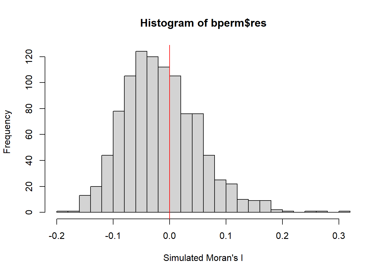
Use ggplot2 package
library(ggplot2)

ggplot(data.frame(Moran_I = bperm$res), aes(x = Moran_I)) +
  geom_histogram(fill = "grey", color = "black") +
  labs(x = "Simulated Moran's I") +
  geom_vline(xintercept = 0, color = "red", linetype = "solid")
`stat_bin()` using `bins = 30`. Pick better value with `binwidth`.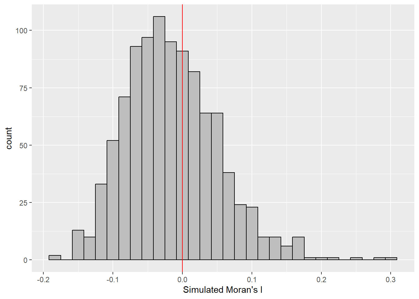
Global Spatial Autocorrelation: Geary’s
Geary’s C test
The code chunk below performs Geary’s C test for spatial autocorrelation by using geary.test() of spdep.
geary.test(hunan$GDPPC, listw=rswm_q)
    Geary C test under randomisation

data:  hunan$GDPPC
weights: rswm_q

Geary C statistic standard deviate = 3.6108, p-value = 0.0001526
alternative hypothesis: Expectation greater than statistic
sample estimates:
Geary C statistic       Expectation          Variance
        0.6907223         1.0000000         0.0073364
Statistically significant, P-value 0.0001526 is less than significance level of 5%.
Computing Monte Carlo Geary’s C
The code chunk below performs permutation test for Geary’s C statistic by using geary.mc() of spdep.
set.seed(1234)
bperm=geary.mc(hunan$GDPPC,
               listw=rswm_q,
               nsim=999)
bperm
    Monte-Carlo simulation of Geary C

data:  hunan$GDPPC
weights: rswm_q
number of simulations + 1: 1000

statistic = 0.69072, observed rank = 1, p-value = 0.001
alternative hypothesis: greater
Statistically significant, P-value 0.0001 is less than significance level of 5%.
Visualising the Monte Carlo Geary’s C
Plot a histogram to reveal the distribution of the simulated values by using the code chunk below.
mean(bperm$res[1:999])[1] 1.004402var(bperm$res[1:999])[1] 0.007436493summary(bperm$res[1:999]) Min. 1st Qu. Median Mean 3rd Qu. Max.
0.7142 0.9502 1.0052 1.0044 1.0595 1.2722 hist(bperm$res, freq=TRUE, breaks=20, xlab="Simulated Geary c")
abline(v=1, col="red") 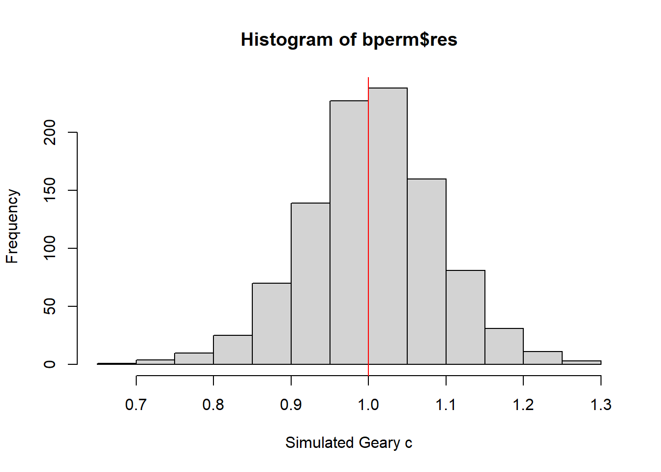
Spatial Correlogram
Compute Moran’s I correlogram
In the code chunk below, sp.correlogram() of spdep package is used to compute a 6-lag spatial correlogram of GDPPC. The global spatial autocorrelation used in Moran’s I.
MI_corr <- sp.correlogram(wm_q,
                          hunan$GDPPC,
                          order=6,
                          method="I",
                          style="W")
plot(MI_corr)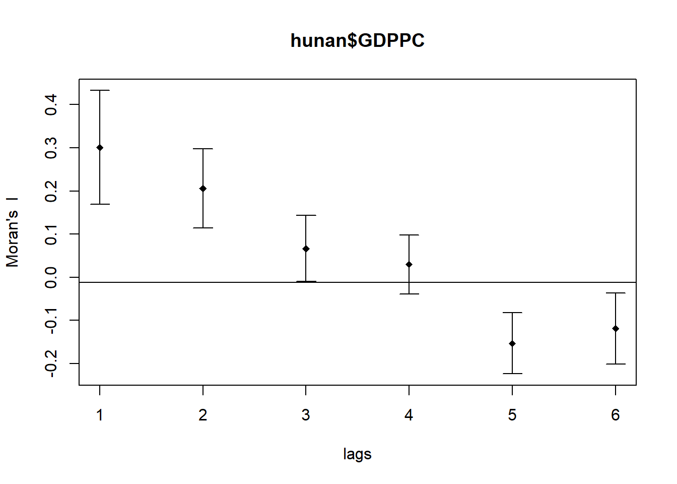
By plotting the output might not allow us to provide complete interpretation. This is because not all autocorrelation values are statistically significant. Hence, it is important for us to examine the full analysis report by printing out the analysis results as in the code chunk below.
print(MI_corr)Spatial correlogram for hunan$GDPPC
method: Moran's I
estimate expectation variance standard deviate Pr(I) two sided
1 (88) 0.3007500 -0.0114943 0.0043484 4.7351 2.189e-06 ***
2 (88) 0.2060084 -0.0114943 0.0020962 4.7505 2.029e-06 ***
3 (88) 0.0668273 -0.0114943 0.0014602 2.0496 0.040400 *
4 (88) 0.0299470 -0.0114943 0.0011717 1.2107 0.226015
5 (88) -0.1530471 -0.0114943 0.0012440 -4.0134 5.984e-05 ***
6 (88) -0.1187070 -0.0114943 0.0016791 -2.6164 0.008886 **
---
Signif. codes: 0 '***' 0.001 '**' 0.01 '*' 0.05 '.' 0.1 ' ' 1Compute Geary’s C correlogram and plot
In the code chunk below, sp.correlogram() of spdep package is used to compute a 6-lag spatial correlogram of GDPPC. The global spatial autocorrelation used in Geary’s C. The plot() of base Graph is then used to plot the output.
GC_corr <- sp.correlogram(wm_q,
                          hunan$GDPPC,
                          order=6,
                          method="C",
                          style="W")
plot(GC_corr)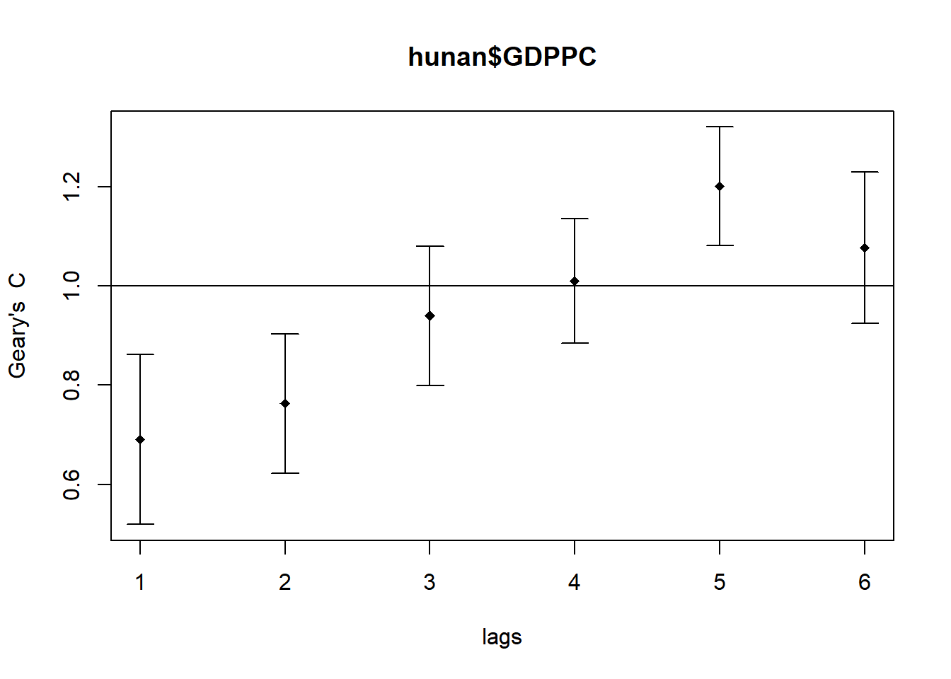
Similar to the previous step, we will print out the analysis report by using the code chunk below.
print(GC_corr)Spatial correlogram for hunan$GDPPC
method: Geary's C
estimate expectation variance standard deviate Pr(I) two sided
1 (88) 0.6907223 1.0000000 0.0073364 -3.6108 0.0003052 ***
2 (88) 0.7630197 1.0000000 0.0049126 -3.3811 0.0007220 ***
3 (88) 0.9397299 1.0000000 0.0049005 -0.8610 0.3892612
4 (88) 1.0098462 1.0000000 0.0039631 0.1564 0.8757128
5 (88) 1.2008204 1.0000000 0.0035568 3.3673 0.0007592 ***
6 (88) 1.0773386 1.0000000 0.0058042 1.0151 0.3100407
---
Signif. codes: 0 '***' 0.001 '**' 0.01 '*' 0.05 '.' 0.1 ' ' 1